#> # A tibble: 4 × 5
#>   term             estimate std.error statistic  p.value
#>   <chr>               <dbl>     <dbl>     <dbl>    <dbl>
#> 1 (Intercept)       -4013.     586.       -6.85 3.74e-11
#> 2 flipper_len          40.6      3.08     13.2  3.64e-32
#> 3 speciesChinstrap   -205.      57.6      -3.57 4.14e- 4
#> 4 speciesGentoo 285. 95.4 2.98 3.08e- 3Statistical
Modeling
Inference and Beyond
R Packages
- Tidyverse
- rcistats
- broom
- emmeans
Palmer Penguins Data
Variables of Interest
species,flipper_lenbody_mass: Body mass in grams

Heart Disease Data
Variables of Interest
cp,trestbpsdisease: Indicating if they have heart disease

Hypothesis Tests: Multi Regression
Hypothesis Tests: Multi Regression
Power Analysis
Simpson’s Paradox
Model Conditions
Hypothesis Tests
Conducting a hypothesis test for coefficients in regression models with more than one predictor is the same as the standard simple approaches.
You will just need to specify the hypothesis tests are adjusted for the other covariates.
Hypothesis Testing Steps
- State \(H_0\) and \(H_1\)
- Choose \(\alpha\)
- Compute confidence interval/p-value
- Make a decision
Null Hypothesis \(H_0\)
The null hypothesis is the claim that is initially believed to be true. For the most part, it is always equal to the hypothesized value.
Alternative Hypothesis \(H_1\)
The alternative hypothesis contradicts the null hypothesis.
Significance Level
Choose a value that represents the probability of being wrong if you decide to reject the \(H_0\).
\[ \alpha = 0.05 \]
Conducting HT of \(\beta_j\) Linear R
XLM: Object where the model is storedY: Name of the outcome variable inDATAX1,X2, …,Xp: predictor variables inDATADATA: Name of the data set
Conducting HT of \(\beta_j\)
XLM: Object where the model is storedY: Name of the outcome variable inDATAX1,X2, …,Xp: predictor variables inDATADATA: Name of the data set
Penguins Example
Is there a significant relationship between penguin body mass (outcome; body_mass) and flipper length (predictor; flipper_len), adjusting for species? Use the penguins data set to determine a significant association.
Penguins: Hypothesis
\(H_0\): There is no relationship between penguin body mass and flipper length, adjusting for penguin species (\(\beta_{flipper\_len} = 0\))
\(H_1\): There is a relationship between penguin body mass and flipper length, adjusting for penguin species (\(\beta_{flipper\_len} \ne 0\))
Penguins: \(\alpha\)-level
\[ \alpha = 0.05 = 5.0*10^{-2} = 5.0e-2 \]
Penguins: Code
Penguins: Decision Making
\[ p = 3.64e-32 < 5e-2 = 0.05 = \alpha \]
Reject \(H_0\)
Penguins: Interpretation
There is a significant association between penguins flipper length and body mass, after adjusting for species (p < 0.0001; \(\beta = 40.7\)). As flipper length increases by 1 unit, body mass increases by 40.7 units, adjusting for penguin species.
Heart Disease Example
Is there a significant association between heart disease (outcome; disease) and resting blood pressure (predictor; trestbps), adjusting for chest pain (cp). Use the heart_disease data set to determine a significant association.
Heart: Hypothesis
\(H_0\): There is no relationship between heart disease probability and resting blood pressure, adjusting for chest pain (\(\beta_{bp} = 0\))
\(H_1\): There is a relationship between heart disease probability and resting blood pressure, adjusting for chest pain (\(\beta_{bp} \ne 0\))
Heart: \(\alpha\)-level
\[ \alpha = 0.05 = 5.0*10^{-2} = 5.0e-2 \]
Heart: Code
#> # A tibble: 5 × 5
#>   term               estimate std.error statistic  p.value
#>   <chr>                 <dbl>     <dbl>     <dbl>    <dbl>
#> 1 (Intercept)         -1.76     1.06        -1.66 9.72e- 2
#> 2 trestbps             0.0209   0.00807      2.59 9.67e- 3
#> 3 cpNon-anginal Pain  -2.28     0.331       -6.87 6.32e-12
#> 4 cpAtypical Angina   -2.45     0.419       -5.85 5.02e- 9
#> 5 cpTypical Angina    -2.04     0.512       -3.99 6.74e- 5
Heart: Decision Making
\[ p = 0.00967 < 0.05 = \alpha \]
Reject \(H_0\)
Heart: Interpretation
There is a significant association between heart disease and resting blood pressure, after adjusting for chest pain (p < 0.00967; \(\beta = 0.0209\)). As resting blood pressure increases by 1 unit, the odds of having heart disease increases by a factor of 1.02, adjusting for chest pain.
Power Analysis
Hypothesis Tests: Multi Regression
Power Analysis
Simpson’s Paradox
Model Conditions
What is Statistical Power
- Statistical Power is the probability of correctly rejecting a false null hypothesis.
- In other words, it’s the chance of detecting a real effect when it exists.
Why Power Matters
- Low power → high risk of Type II Error (false negatives)
- High power → better chance of finding true effects
- Common threshold: 80% power
Errors in Inference
| Type I | Reject \(H_0\) when true | False positive |
| Type II | Don’t reject \(H_0\) when false | False negative |
| Power | \(1 - P(\text{Type II})\) | Detecting a true effect |
Type I Error (False Positive)
- Rejecting \(H_0\) when it is actually true
- Probability = \(\alpha\) (significance level)
Type II Error (False Negative)
- Failing to reject \(H_0\) when it is actually false
- Probability = \(\beta\)
- Power = \(1 - \beta\)
Balancing Errors
- Lowering \(\alpha\) reduces Type I errors, but increases risk of Type II errors.
- To reduce both:
- Increase sample size
- Use more appropriate statistical tests
What Affects Power?
- Effect Size
- Bigger effects are easier to detect
- Sample Size (\(n\))
- Larger samples reduce standard error
- Significance Level (\(\alpha\))
- Higher \(\alpha\) increases power (but riskier!)
- Variability
- Less noise in data = better power
Boosting Power
- Power = Probability of rejecting \(H_0\) when it’s false
- Helps avoid Type II Errors
- Driven by:
- Sample size
- Effect size
- \(\alpha\)
- Variability
- Aim for 80% or higher
Simpson’s Paradox
Hypothesis Tests: Multi Regression
Power Analysis
Simpson’s Paradox
Model Conditions
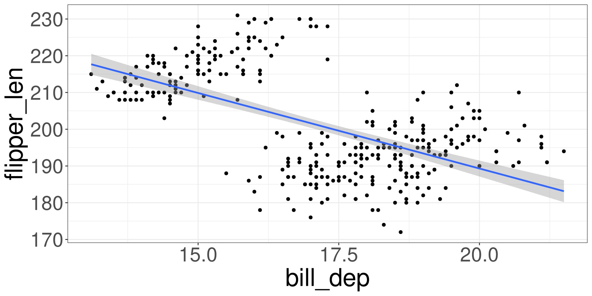
Penguins Bill Depth vs Flipper Length
Penguins Bill Depth vs Flipper Length by Species
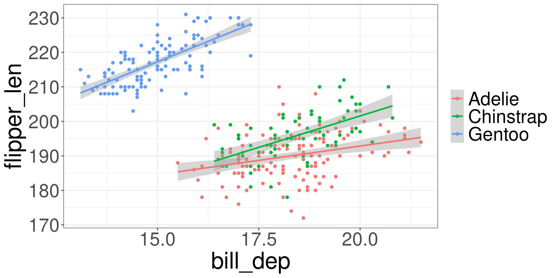
Simpson’s Paradox
Simpson’s paradox is a phenomenon in probability and statistics in which a trend appears in several groups of data but disappears or reverses when the groups are combined.
Model Conditions
Hypothesis Tests: Multi Regression
Power Analysis
Simpson’s Paradox
Model Conditions
Model Conditions
When we are conducting inference with regression models, we will have to check the following conditions:
- Linearity
- Independence
- Probability Assumption
- Equal Variances
- Multicollinearity (for Multi-Regression)
Linearity
There must be a linear relationship between both the outcome variable (y) and a set of predictors (\(x_1\), \(x_2\), …).
Independence
The data points must not influence each other.
Probability Assumption
The model errors (also known as residuals) must follow a specified distribution.
Linear Regression: Normal Distribution
Logistic Regression: Binomial Distribution
Equal Variances
The variability of the data points must be the same for all predictor values.
Residuals
Residuals are the errors between the observed value and the estimated model. Common residuals include
Raw Residual
Standardized Residuals
Jackknife (studentized) Residuals
Deviance Residuals
Quantized Residuals
Influential Measurements
Influential measures are statistics that determine how much a data point affects the model. Common influential measures are
Leverages
Cook’s Distance
Raw Residuals
\[ \hat r_i = y_i - \hat y_i \]
Residual Analysis
A residual analysis is used to test the assumptions of linear regression.
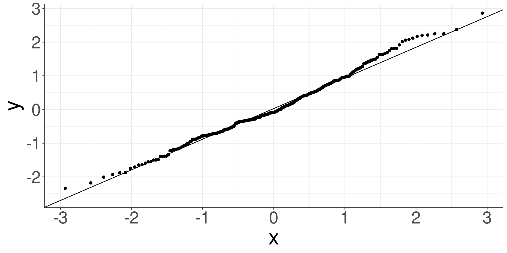
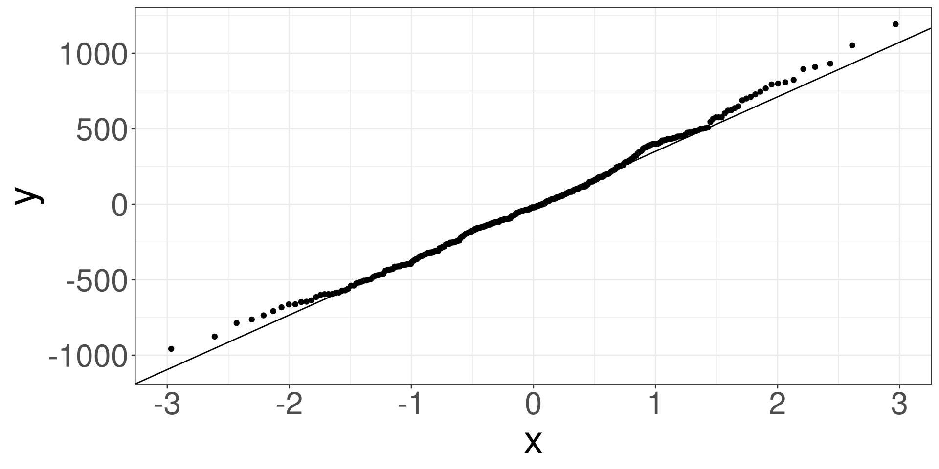
QQ Plot
A qq (quantile-quantile) plot will plot the estimated quantiles of the residuals against the theoretical quantiles from a normal distribution function. If the points from the qq-plot lie on the \(y=x\) line, it is said that the residuals follow a normal distribution.
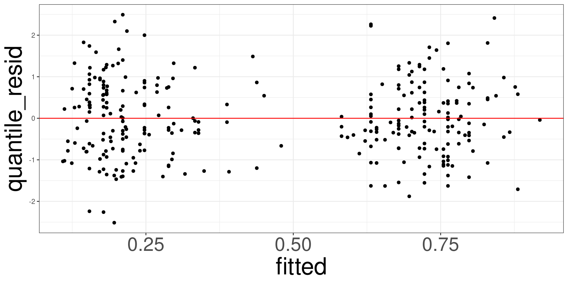
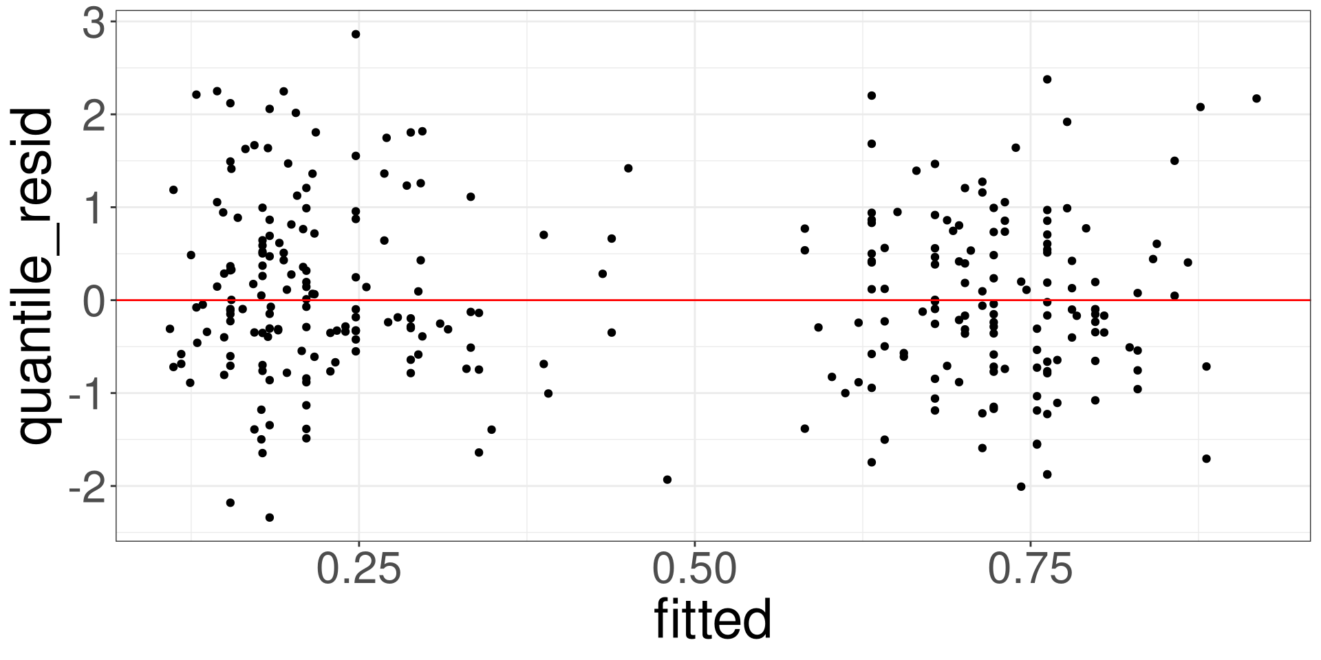
Residual vs Fitted Plot
This plot allows you to assess the linearity, constant variance, and identify potential outliers. Create a scatter plot between the fitted values (x-axis) and the raw/standardized residuals (y-axis).
Residual Analysis in R
Use the resid_df function to obtain the residuals of a model.
Residual vs Fitted Plot
Linear
Logistic
RDF: Name of object fromresid_df()
QQ Plot
Linear
Logistic
RDF: Name of object fromresid_df()
Penguins: Example
#>   obs body_mass    island species flipper_len       resid   fitted     sresid
#> 1   1      3750 Torgersen  Adelie         181  474.240098 3275.760  1.2893948
#> 2   2      3800 Torgersen  Adelie         186  318.792779 3481.207  0.8642963
#> 3   3      3250 Torgersen  Adelie         195 -601.012396 3851.012 -1.6283711
#> 4   4      3450 Torgersen  Adelie         193 -318.833468 3768.833 -0.8635409
#> 5   5      3650 Torgersen  Adelie         190    4.434923 3645.565  0.0120118
#> 6   6      3625 Torgersen  Adelie         181  349.240098 3275.760  0.9495367
#>      hatvals   jackknife        cooks
#> 1 0.02891587  1.29070703 8.250875e-03
#> 2 0.02338420  0.86396116 2.981074e-03
#> 3 0.02210495 -1.63251165 9.989709e-03
#> 4 0.02142503 -0.86320431 2.721084e-03
#> 5 0.02143822  0.01199342 5.268237e-07
#> 6 0.02891587  0.94939343 4.474573e-03
Penguins: Residual vs Fitted Plots
Penguins: QQ Plot
Heart: Example
Code
#>   obs disease trestbps               cp    fitted        eta  raw_resid
#> 1   1      no      145   Typical Angina 0.3162617 -0.7710053 -0.3162617
#> 2   2     yes      160     Asymptomatic 0.8296967  1.5834796  0.1703033
#> 3   3     yes      120     Asymptomatic 0.6787886  0.7482102  0.3212114
#> 4   4      no      130 Non-anginal Pain 0.2107532 -1.3203915 -0.2107532
#> 5   5      no      130  Atypical Angina 0.1834250 -1.4933128 -0.1834250
#> 6   6      no      120  Atypical Angina 0.1541873 -1.7021301 -0.1541873
#>   pearson_resid deviance_resid working_resid partial_resid.trestbps
#> 1    -0.6801087     -0.8719863     -2.233553              -1.184687
#> 2     0.4530559      0.6110565      2.788739               1.796346
#> 3     0.6879046      0.8802790      2.221423               1.229030
#> 4    -0.5167502     -0.6880061     -2.587422              -1.302396
#> 5    -0.4739486     -0.6366106     -2.717940              -1.259993
#> 6    -0.4269600     -0.5787181     -2.884425              -1.426478
#>   partial_resid.cp std_pear_resid std_dev_resid stud_dev_resid quantile_resid
#> 1        -2.305014     -0.6962858    -0.8927274     -0.8846616   -0.313701994
#> 2         2.404052      0.4562301     0.6153377      0.6134136    0.076564332
#> 3         2.672005      0.6910541     0.8843093      0.8827424   -0.003954837
#> 4        -2.345657     -0.5199246    -0.6922325     -0.6903935   -0.289474352
#> 5        -2.476175     -0.4789686    -0.6433536     -0.6403567   -1.345472186
#> 6        -2.433842     -0.4311339    -0.5843756     -0.5818043   -0.095807259
#>     leverages        cooks
#> 1 0.045927133 0.0046675922
#> 2 0.013866647 0.0005853744
#> 3 0.009094376 0.0008765864
#> 4 0.012173676 0.0006662724
#> 5 0.020852010 0.0009771107
#> 6 0.019268922 0.0007304018
Heart: Residual vs Fitted Plots
Heart: QQ Plot