Inference with Linear Regression
2025-04-21
Motivating Example

Standard Normal Distribution
\[ {\frac{1}{\sqrt{2 \pi}}} e^{-\frac{1}{2}x^2} \]
Code
data.frame(x = seq(-5,5, length.out = 100),
           y1 = dt(seq(-5,5, length.out = 100), 1),
           y2 = dt(seq(-5,5, length.out = 100), 10),
           y3 = dt(seq(-5,5, length.out = 100), 30),
           y4 = dt(seq(-5,5, length.out = 100), 100),
           y5 = dnorm((seq(-5,5, length.out = 100)))) |>
  ggplot() +
  # geom_line(aes(x, y1, color = "1")) +
  # geom_line(aes(x, y2, color = "10")) +
  # geom_line(aes(x, y3, color = "30")) +
  # geom_line(aes(x, y4, color = "100")) +
  geom_line(aes(x, y5)) +
  ylab("y")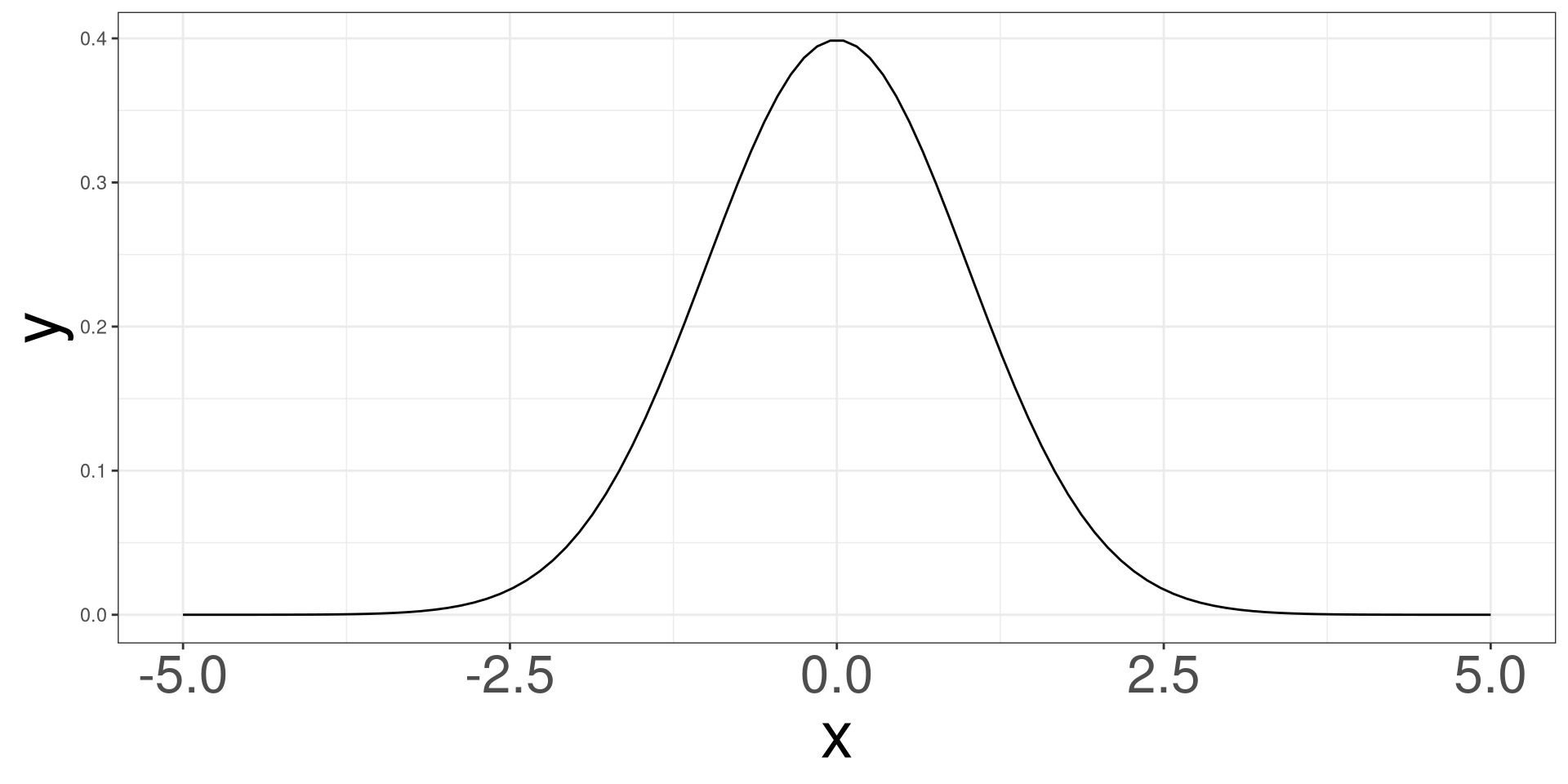
t Distribution
\[ \frac{\Gamma \left(\frac{v+1}{2}\right)}{\sqrt{\pi v}\Gamma\left(\frac{v}{2}\right)} \left(1 + \frac{x^2}{v}\right)^{-\frac{v+1}{2}} \]
Code
data.frame(x = seq(-5,5, length.out = 100),
           y1 = dt(seq(-5,5, length.out = 100), 1),
           y2 = dt(seq(-5,5, length.out = 100), 10),
           y3 = dt(seq(-5,5, length.out = 100), 30),
           y4 = dt(seq(-5,5, length.out = 100), 100),
           y5 = dnorm((seq(-5,5, length.out = 100)))) |>
  ggplot() +
  geom_line(aes(x, y1, color = "1")) +
  geom_line(aes(x, y2, color = "10")) +
  geom_line(aes(x, y3, color = "30")) +
  geom_line(aes(x, y4, color = "100")) +
  geom_line(aes(x, y5, color = "Normal")) +
  ylab("y")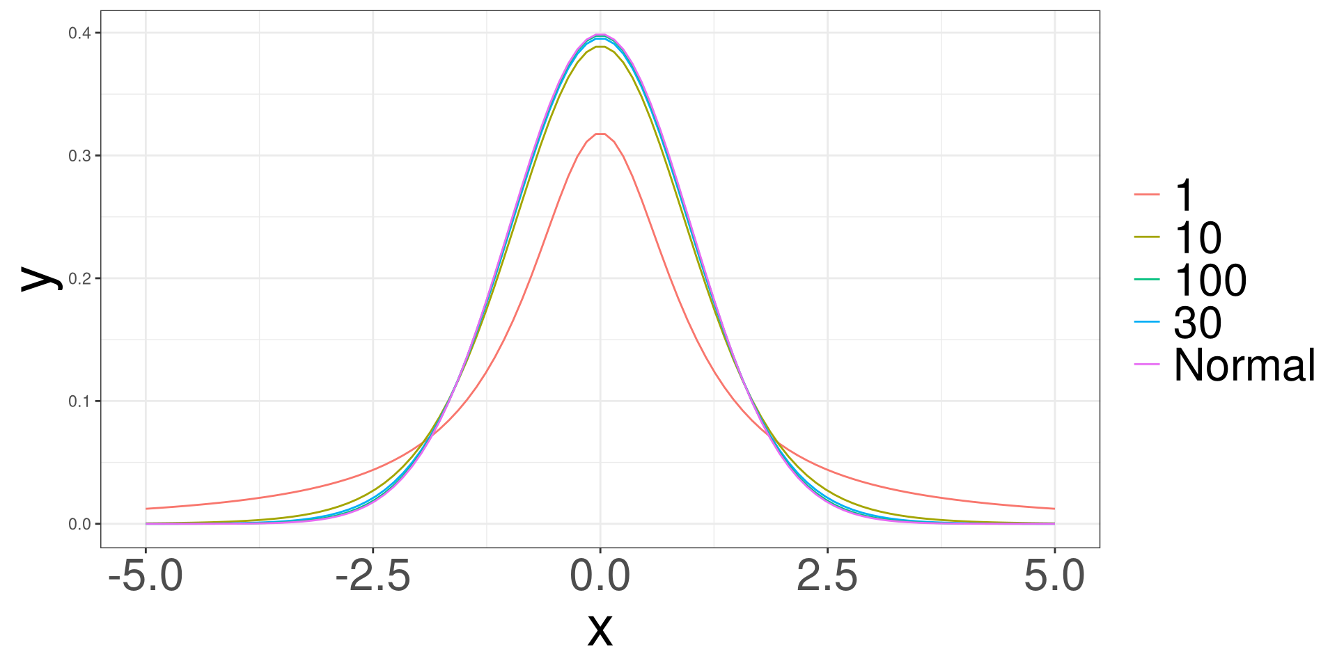
Example