Simple
Linear Regression

R Packages

• rcistats
• tidyverse

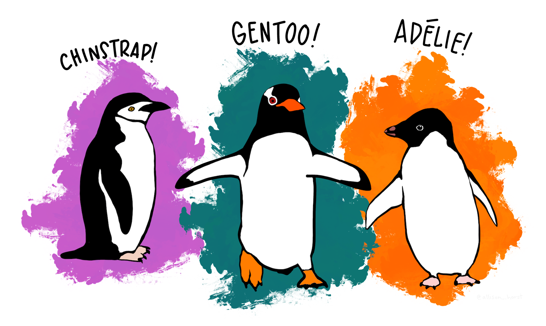
Palmer Penguins Data

Variables of Interest

• flipper_len: Flipper Length in millimeters
• body_mass: Body mass in grams

Artwork by @allison_horst

Variables of Interest

Modeling Relationships

• Modeling Relationships

• A Simple Model

• Modelling Data

• Linear Model

• Prediction

Explaining Variation

This is the process where we try to reduce the variation with the use of other variables.

Can be thought of as getting it less wrong when taking an educated guess.

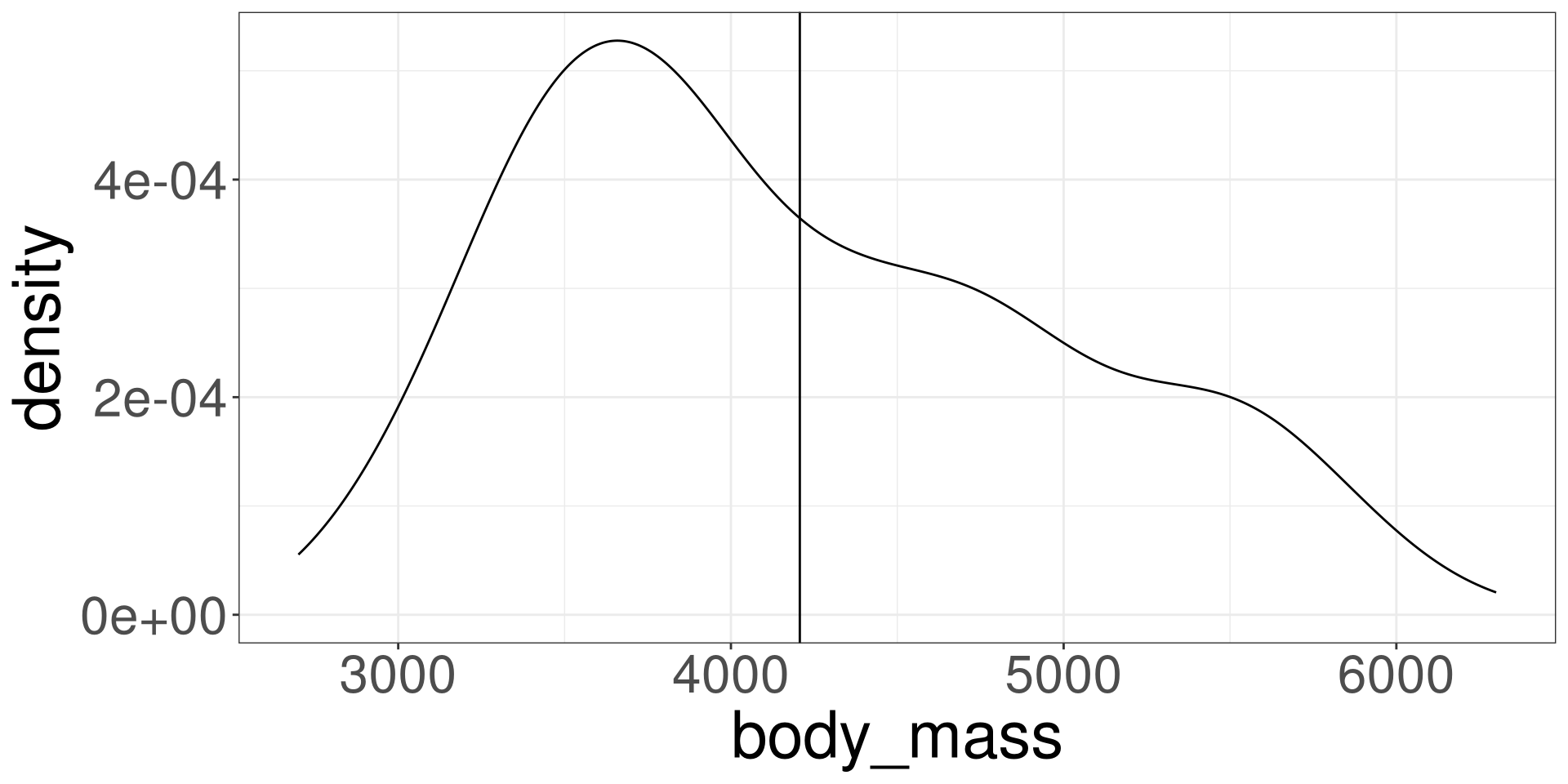
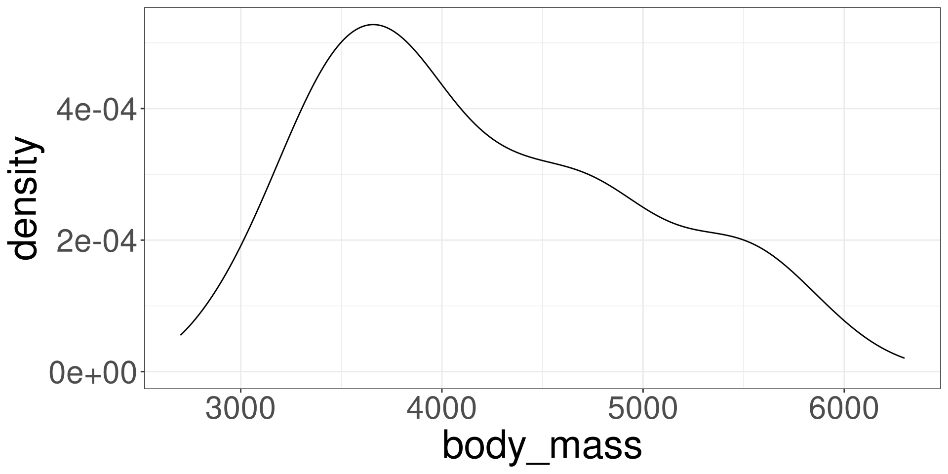
Modeling Variation

ggplot(penguins, aes(body_mass)) +
  geom_density() 

Modeling Variation with \(\bar X\)

ggplot(penguins, aes(body_mass)) +
  geom_density() +
  geom_vline(xintercept = mean(penguins$body_mass))

Modeling with a Numerical Variable

ggplot(penguins, aes(x = flipper_len, y = body_mass)) +
  geom_point() +
  stat_density_2d(aes(fill = after_stat(level))) +
  xlim(c(170, 236)) +
  ylim(c(2500, 6250))

Modeling with a Numerical Variable

ggplot(penguins, aes(x = flipper_len, y = body_mass)) +
  geom_point() +
  stat_smooth(method = "lm", se = F, col = "red") +
  stat_density_2d(aes(fill = after_stat(level))) +
  xlim(c(170, 236)) +
  ylim(c(2500, 6250))

A Simple Model

• Modeling Relationships

• A Simple Model

• Modelling Data

• Linear Model

• Prediction

Generated Model

\[ Y \sim DGP_1 \]

A Simple Model

ggplot(penguins, aes(body_mass)) +
  geom_density()

A Simple Model

\[ Y = \_\_\_ + error \]

Notation

\[ Y = \ \ \ \ \ \ \ \ \ + \varepsilon \]

The Simple Generated Model

\[ Y \sim \beta_0 + \varepsilon \]

\[ \varepsilon \sim DGP_2 \]

\(DGP_2\) is not the same as the \(DGP_1\), it is transformed due \(\beta_0\). Consider this the NULL \(DGP\).

Observing Data

\[ Y = \beta_0 + \varepsilon \]

Estimated Line

\[ \hat Y=\hat\beta_0 \]

Notation

Observed

\[ Y = \beta_0 + \varepsilon \]

Estimated

\[ \hat Y = \hat \beta_0 \]

Modelling Data

• Modeling Relationships

• A Simple Model

• Modelling Data

• Linear Model

• Prediction

Indexing Data

The data in a data set can be indexed by a number.

penguins[1,-c(1:2)]

#>   bill_len bill_dep flipper_len body_mass  sex year
#> 1     39.1     18.7         181      3750 male 2007

Making the variable body_mass be represented by \(Y\) and flipper_len as \(X\):

\[ Y_1 = 3750 \ \ X_1=181 \]

Indexing Data

\[ Y_i, X_i \]

Data

With the data that we collect from a sample, we hypothesize how the data was generated.

Using a simple model:

\[ Y_i = \beta_0 + \varepsilon_i \]

Estimated Value

\[ \hat Y_i = \hat \beta_0 \]

Estimation

To estimate \(\hat \beta_0\), we minimize the follow function:

\[ \sum^n_{i=1} (Y_i-\hat Y_i)^2 \]

This is known as the sum squared errors, SSE

Residuals

The residuals are known as the observed errors from the data in the model:

\[ r_i = Y_i - \hat Y_i \]

Estimation in R

lm(Y ~ 1, data = DATA)

• Y: Name Outcome Variable of Interest in data frame DATA
• DATA: Name of the data frame

Modeling Body Mass in Penguins

xlm <- lm(body_mass ~ 1, data = penguins)
xlm

#> 
#> Call:
#> lm(formula = body_mass ~ 1, data = penguins)
#> 
#> Coefficients:
#> (Intercept)  
#>        4207

\[ \hat Y = 4207 \]

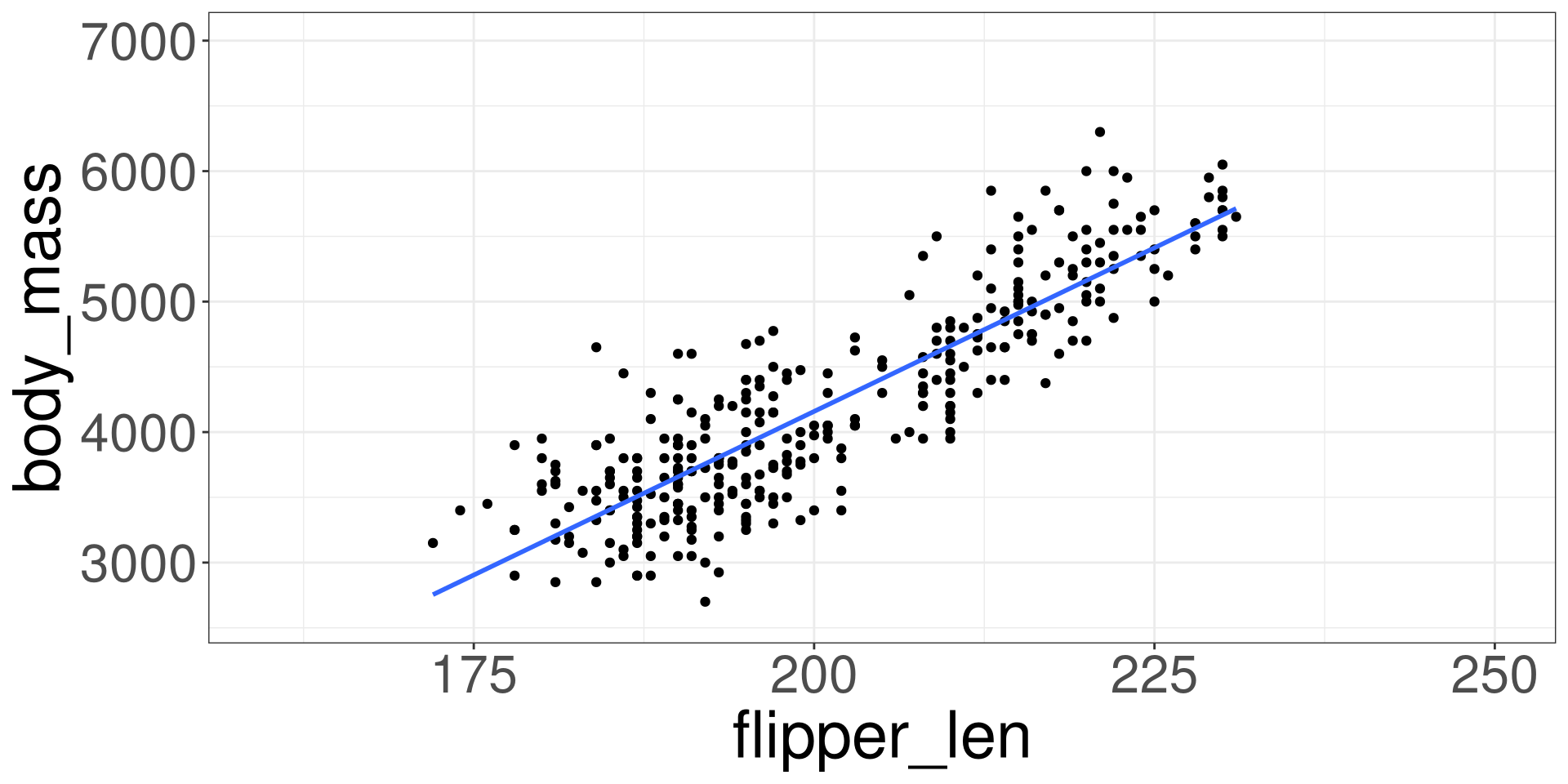
Visualize

ggplot(penguins, aes(body_mass)) +
  geom_density() +
  geom_vline(xintercept = 4207)

Linear Model

• Modeling Relationships

• A Simple Model

• Modelling Data

• Linear Model

• Prediction

Linear Model

The goal of Statistics is to develop models the have a better explanation of the outcome \(Y\).

In particularly, reduce the sum of squared errors.

By utilizing a bit more of information, \(X\), we can increase the predicting capabilities of the model.

Thus, the linear model is born.

Visualization

• 1-Dimensional
• 2-Dimensional

ggplot(penguins, aes(body_mass)) +
  geom_density()

ggplot(penguins, aes(x = flipper_len, y = body_mass)) +
  geom_point() +
  stat_density_2d(aes(fill = after_stat(level))) +
  xlim(c(170, 236)) +
  ylim(c(2500, 6250))

Linear Model

\[ Y = \beta_0 + \beta_1 X + \varepsilon \]

\[ \varepsilon \sim DGP_3 \]

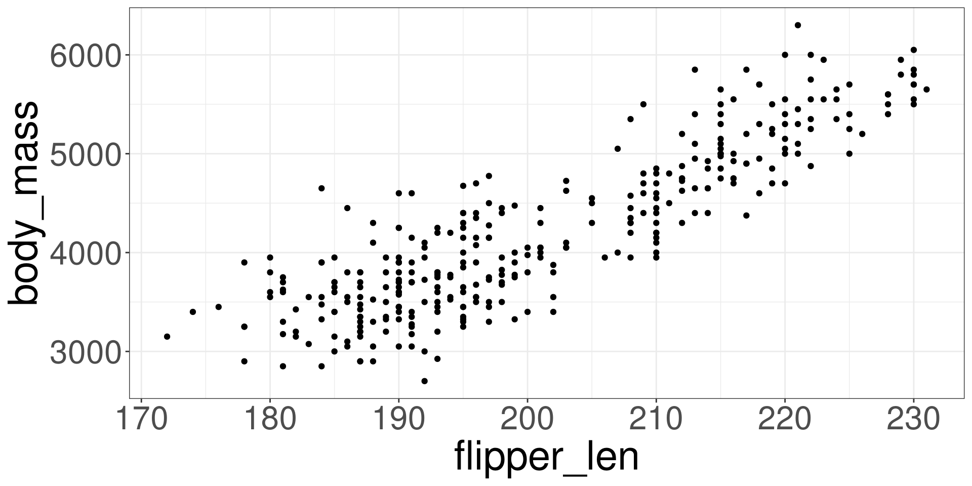
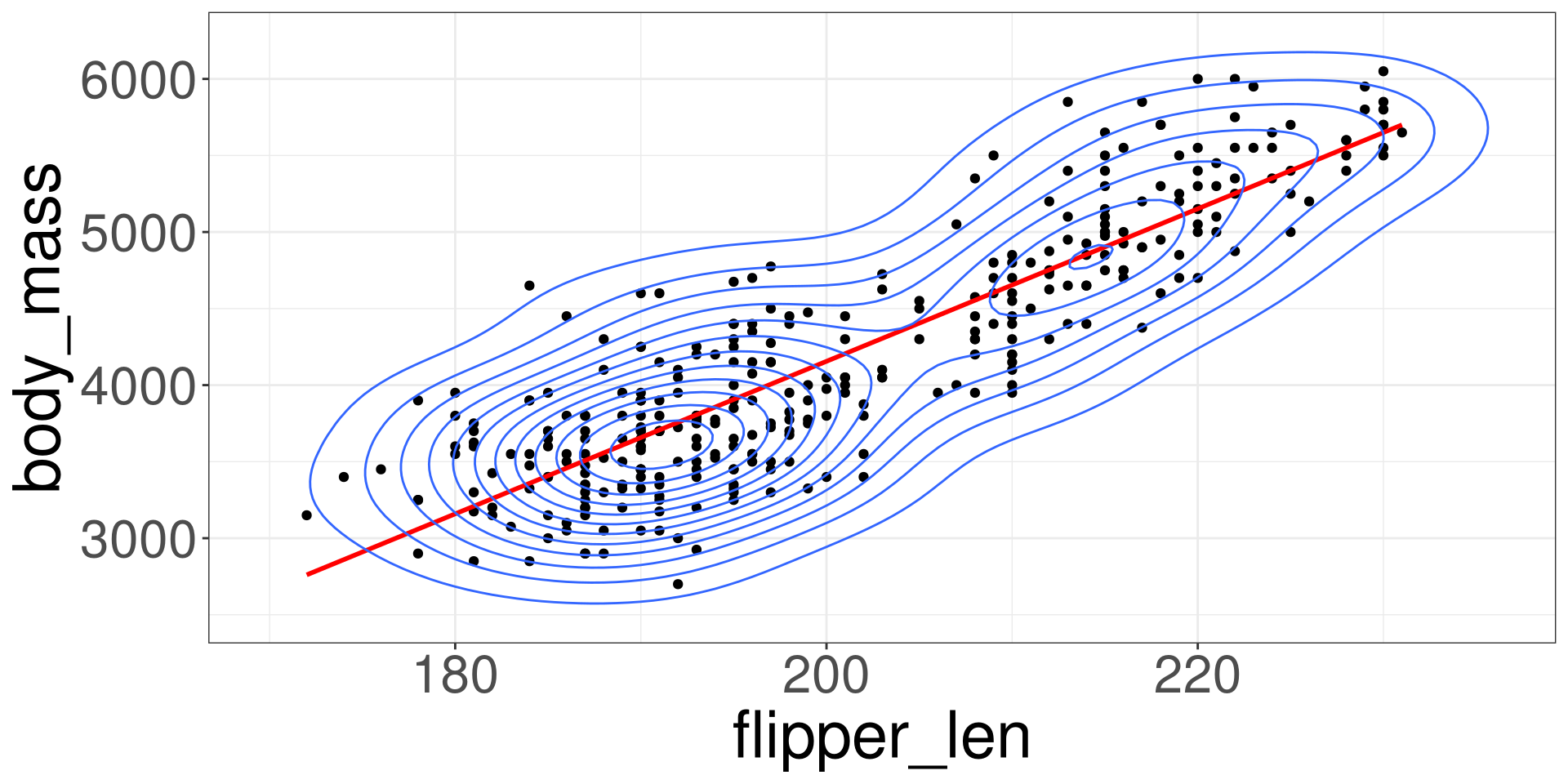
Scatter Plot

ggplot(penguins, aes(flipper_len, body_mass)) + 
  geom_point() 

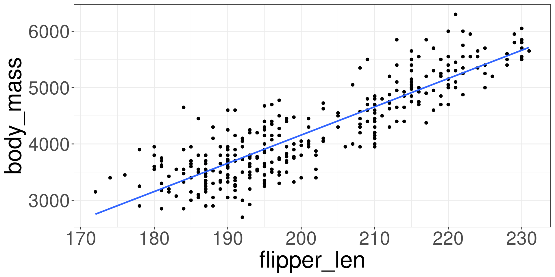
Imposing a Line

ggplot(penguins, aes(flipper_len, body_mass)) + 
  geom_point() +
  stat_smooth(method = "lm", se = F) 

Modelling the Data

\[ Y_i = \beta_0 + \beta_1 X_i + \varepsilon_i \]

Linear Model

\[ \hat Y_i = \hat \beta_0 + \hat \beta_1 X_i \]

Goal is to obtain numerical values for \(\hat \beta_0\) and \(\hat \beta_1\) that will minimize the SSE.

SSE

\[ \sum^n_{i=1} (Y_i-\hat Y_i)^2 \]

\[ \hat Y_i = \hat \beta_0 + \hat \beta_1 X_i \]

Fitting a Model in R

xlm <- lm(Y ~ X, data = DATA)
xlm

• X: Name Predictor Variable of Interest in data frame DATA
• Y: Name Outcome Variable of Interest in data frame DATA
• DATA: Name of the data frame

Example

Y: body_mass; X: flipper_len

xlm <- lm(body_mass ~ flipper_len, data = penguins)
xlm

#> 
#> Call:
#> lm(formula = body_mass ~ flipper_len, data = penguins)
#> 
#> Coefficients:
#> (Intercept)  flipper_len  
#>    -5872.09        50.15

\[ \hat Y_i = -5872.09 + 50.15 X_i \]

Interpretation of \(\hat\beta_0\)

The intercept \(\hat \beta_0\) can be interpreted as the base value when \(X\) is set to 0.

Some times the intercept can be interpretable to real world scenarios.

Other times it cannot.

Interpreting Example

\[ \hat Y_i = -5872.09 + 50.15 X_i \]

When flipper length is 0 mm, the body mass is -5872 grams.

Interpretation of \(\hat \beta_1\)

The slope \(\hat \beta_1\) indicates how will y change when x increases by 1 unit.

It will demonstrate if there is, on average, a positive or negative relationship based on the sign provided.

Interpreting Example

\[ \hat Y_i = -5872.09 + 50.15 X_i \]

When flipper length increases by 1 mm, the body mass will increase by 50.15 grams.

Prediction

• Modeling Relationships

• A Simple Model

• Modelling Data

• Linear Model

• Prediction

Statistical Model

\[ \hat Y = \hat \beta_0 + \hat \beta_1 X \]

• \(X\): Input
• \(\hat Y\): Output

Prediction

Using the equation \(\hat Y\), we can give it a value of \(X\) and then, in return, a value of \(\hat Y\) that predicts the true value \(Y\).

Prediction in R

xlm <- lm(Y ~ X,
            data = DATA)

predict_df <- data.frame(X = VAL)

predict(xlm,
        predict_df)

• X: Name Predictor Variable of Interest in data frame DATA
• Y: Name Outcome Variable of Interest in data frame DATA
• DATA: Name of the data frame
• VAL: Value for the Predictor Variable

Example 1

• Example
• Code

Predict the body mass for a penguin with a flipper length of 185.

xlm <- lm(body_mass ~ flipper_len,
            data = penguins)

xlm

#> 
#> Call:
#> lm(formula = body_mass ~ flipper_len, data = penguins)
#> 
#> Coefficients:
#> (Intercept)  flipper_len  
#>    -5872.09        50.15

predict_df <- data.frame(flipper_len = 185)

predict(xlm,
        predict_df)

#>        1 
#> 3406.262

Example 2

• Example
• Code

Predict the body mass for a penguin with a flipper length of 205.

xlm <- lm(body_mass ~ flipper_len,
            data = penguins)


xlm

#> 
#> Call:
#> lm(formula = body_mass ~ flipper_len, data = penguins)
#> 
#> Coefficients:
#> (Intercept)  flipper_len  
#>    -5872.09        50.15

predict_df <- data.frame(flipper_len = 190)

predict(xlm,
        predict_df)

#>        1 
#> 3657.028

Interpolation

Interpolation is the process of estimating a value within the range of the observed input data \(X\).

Extrapolation

Extrapolation is the process of estimating a value beyond the range of observed input data \(X\). It’s about venturing into the unknown, using what we know as a guide.

Extrapolation

ggplot(penguins, aes(flipper_len, body_mass)) + 
  xlim(160, 250) +
  ylim(2600, 7000) +
  geom_point() +
  stat_smooth(method = "lm", se = F)