Multivariable
Regression
Palmer Penguins Data
Variables of Interest
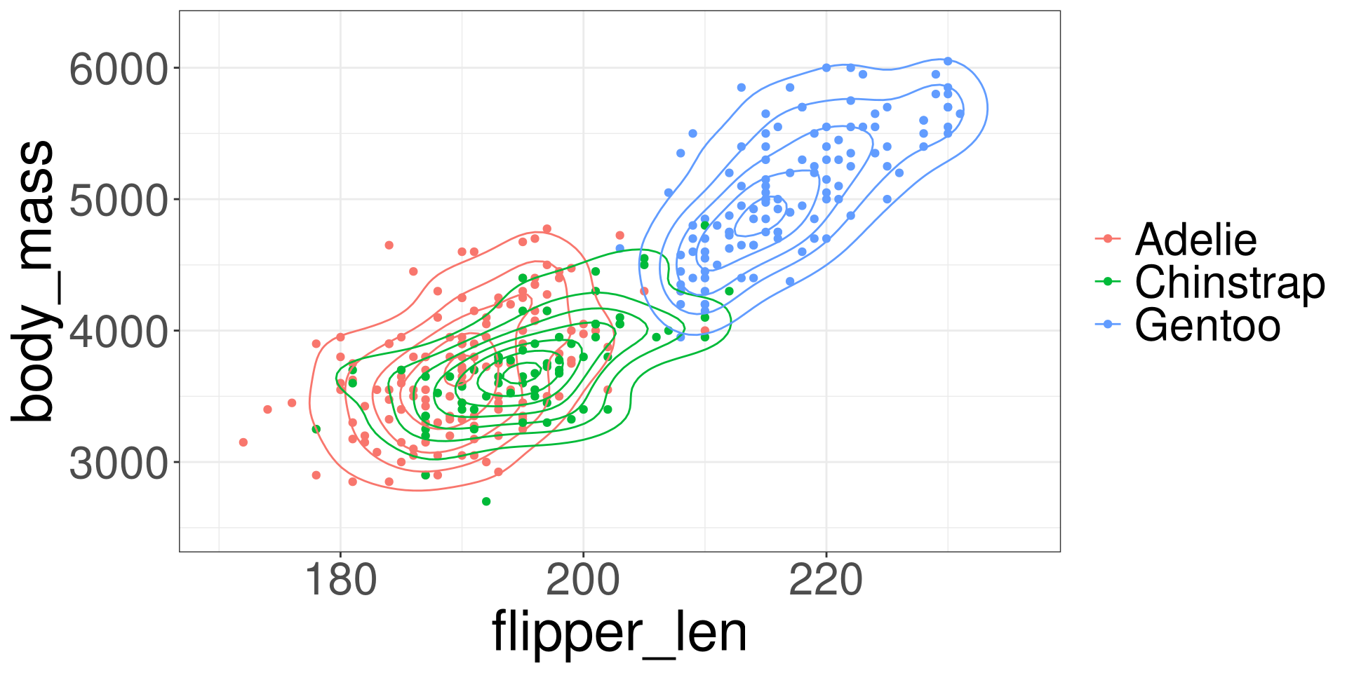
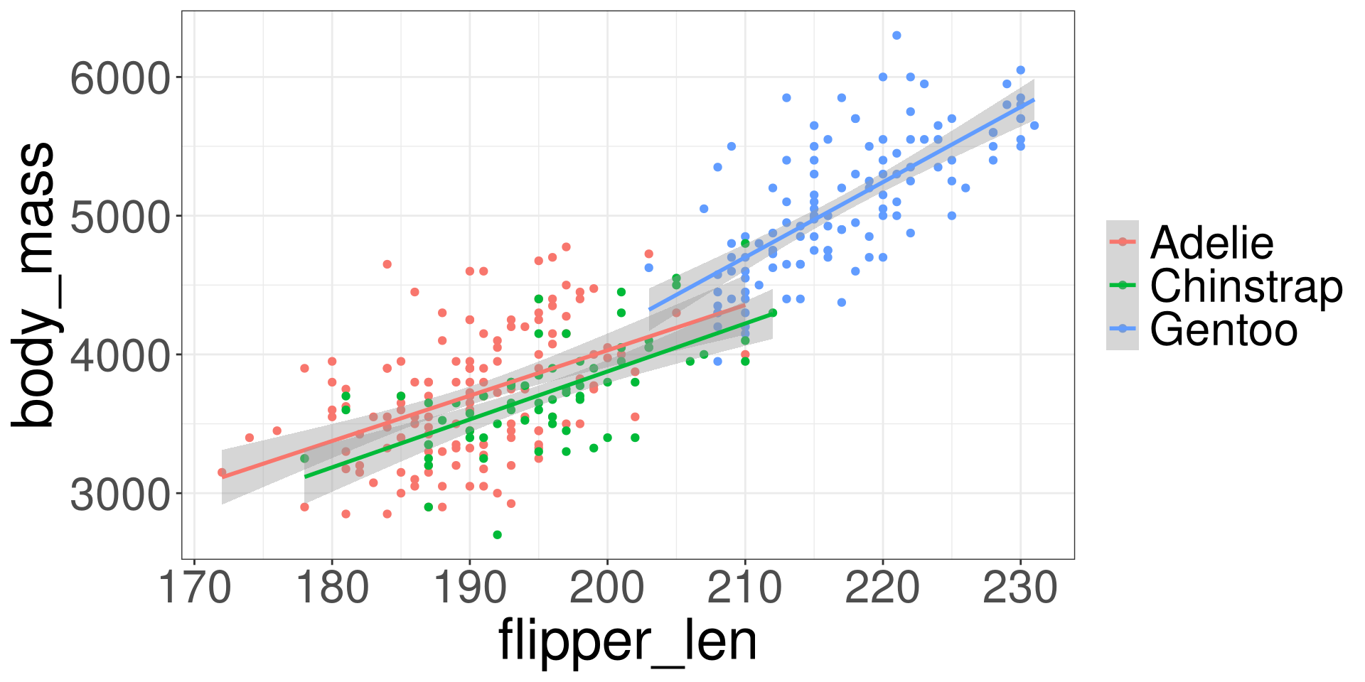
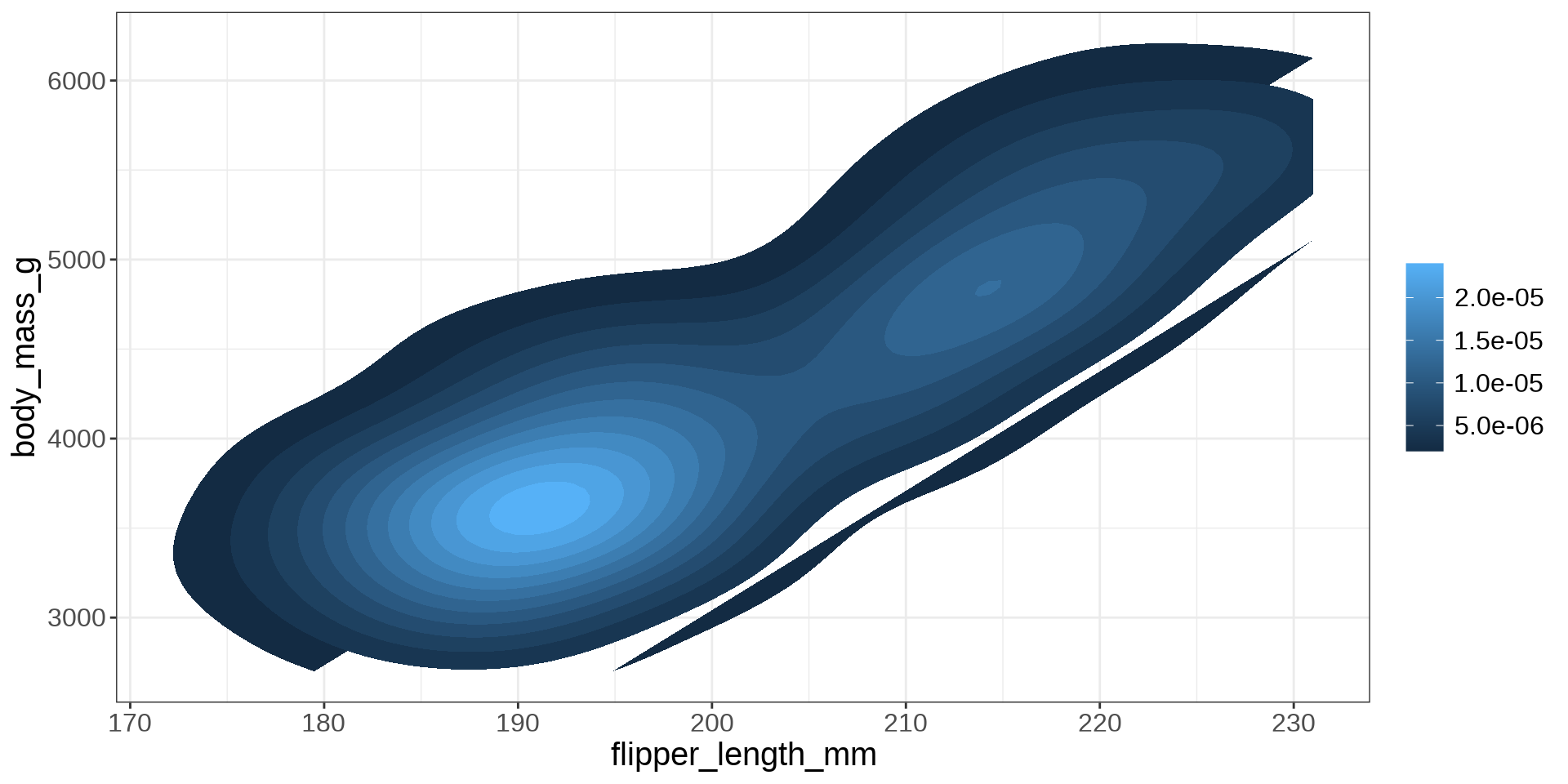
species: Penguin speciesflipper_len: Flipper Length in millimetersbody_mass: Body mass in grams

Heart Disease Data
Variables of Interest
thal: Thallium stress test resultthalach: Maximum heart rate achieveddisease: Indicating if they have heart disease

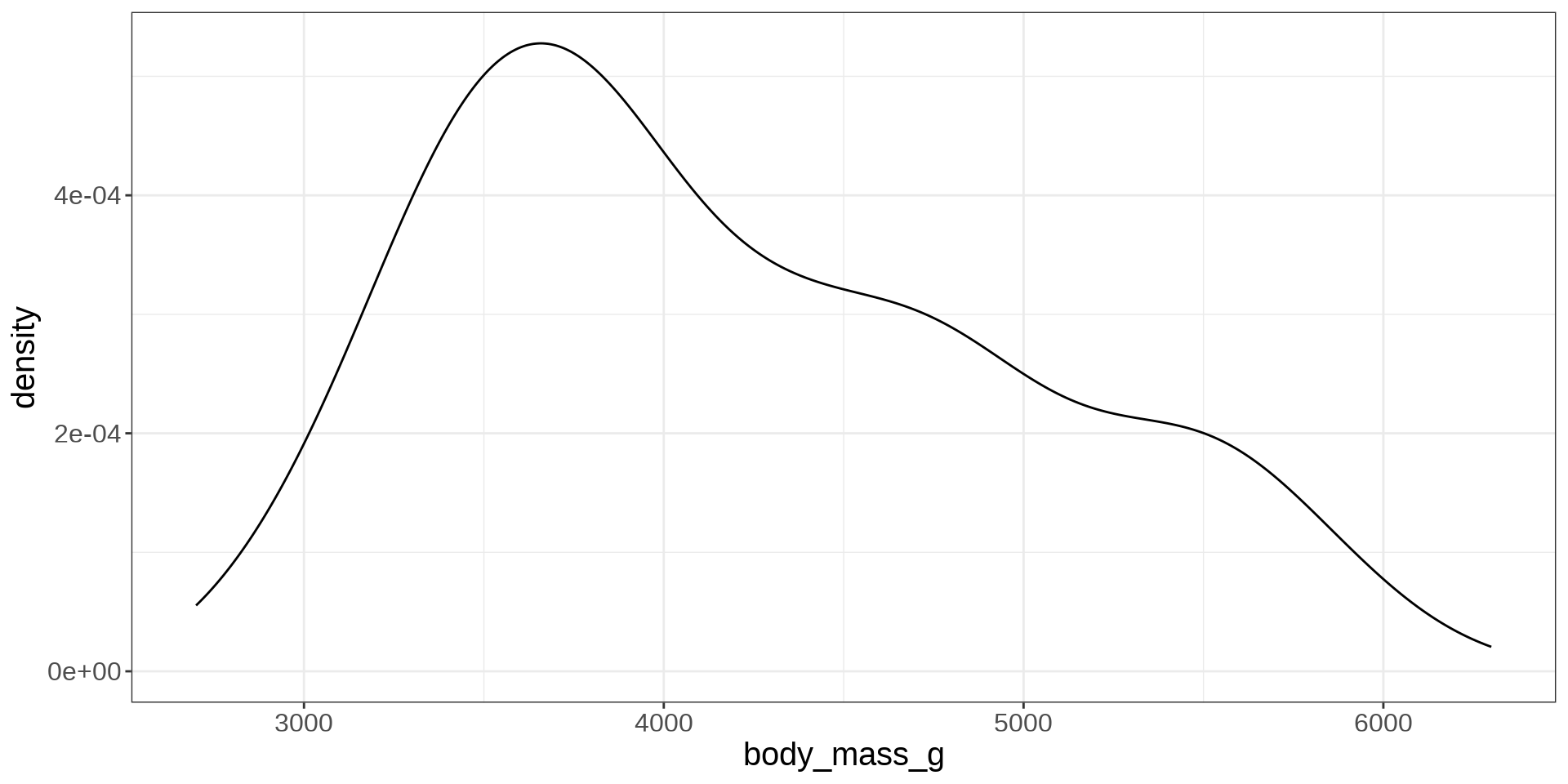
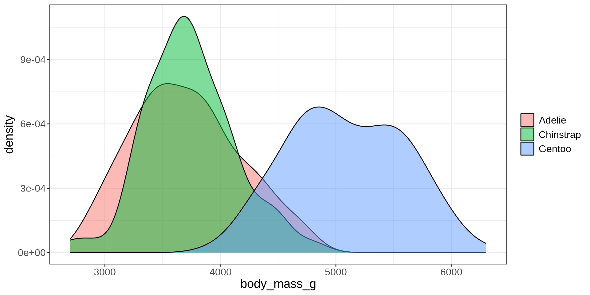
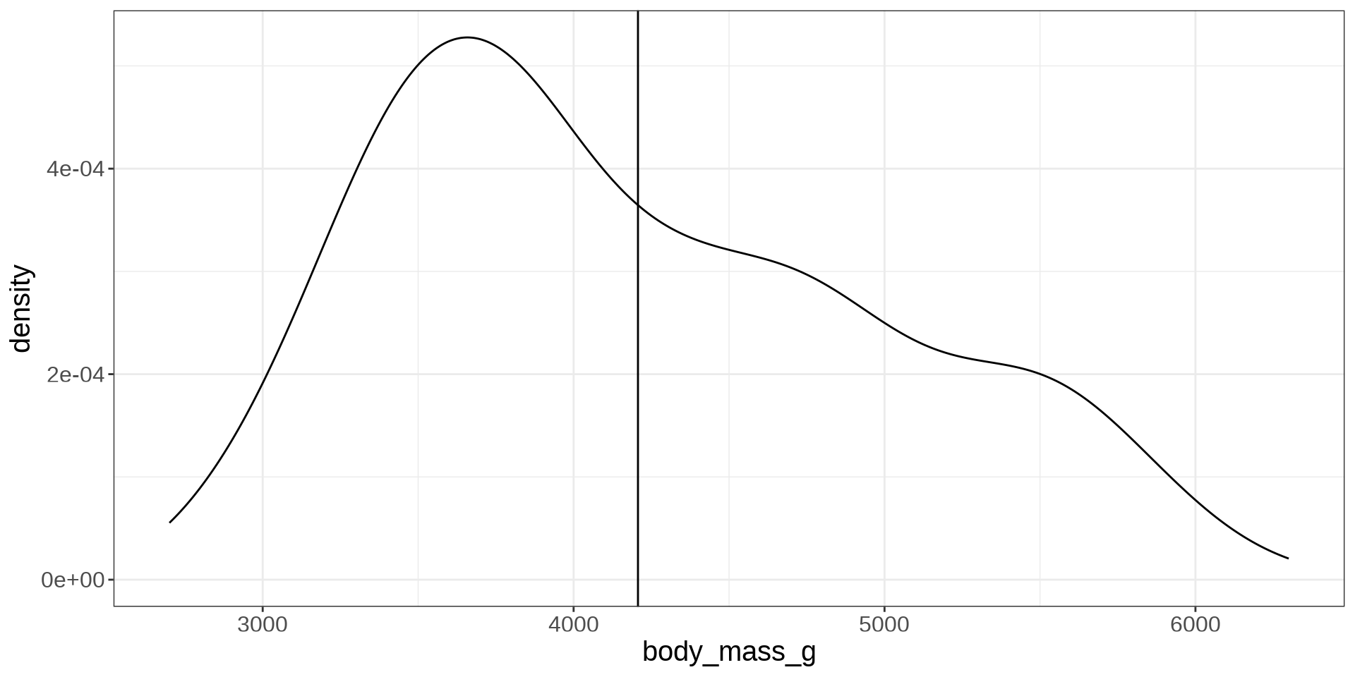
Penguins: Body Mass

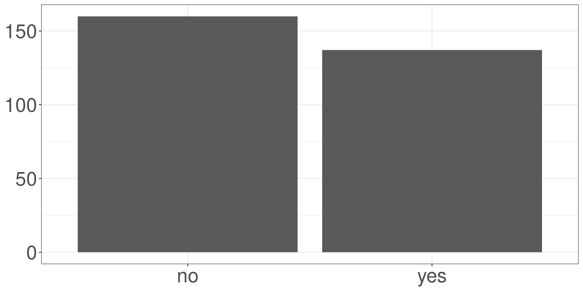
Heart Disease

About Model Selection
Generally, it is not a good idea to conduct model selection. The predictor variables in your model should be guided by a literature review that illustrates important predictor variables in a model. Add predictor variables based on consultation with experts and a literature review.