# This code will load the R packages we will use
install.packages(c("rcistats"),
                 repos = c("https://inqs909.r-universe.dev", "https://cloud.r-project.org"))
library(rcistats)
library(tidyverse)


# Uncomment and run for themes
# rcistats::install_themes()
# library(ThemePark)
# library(ggthemes)Categorical Data
Descriptive summaries & visualizations (freq, proportion, crosstabs, bar/pie/mosaic/waffle)
1 Introduction
- Recognize and work with categorical variables in R.
- Summarize categories using frequencies and proportions (a.k.a. relative frequency).
- Create standard plots for categorical data: bar, stacked bar, pie, mosaic, and waffle.K
- Read and interpret cross‑tabulations (two‑way tables) with row/column/table proportions.
Tip
Use the Copy button on each code chunk. Many chunks include a template version followed by a worked example.
2 Google Colab Setup
Copy the following code and put it in a code cell in Google Colab. Only do this if you are using a completely new notebook.
2.1 Data for this handout
We will use the Great American Coffee Taste Test survey data from TidyTuesday. Below is a subset of the data.
Code
coffee <- read_csv("https://raw.githubusercontent.com/rfordatascience/tidytuesday/master/data/2024/2024-05-14/coffee_survey.csv")2.2 Using the templates: what to change
Use this legend whenever you see a Template code block.
DATA→ replace with your data frame/tibble name (e.g.,coffee).VAR→ replace with the single categorical variable you want (e.g.,caffeine).- In
ggplot(DATA, aes(x = VAR)), writeggplot(coffee, aes(x = caffeine)). - In functions that take a vector (e.g.,
cat_stats(DATA$VAR)), writecat_stats(coffee$caffeine).
- In
VAR1andVAR2→ replace with the first and second categorical variables for two‑way tables/stacked bars (e.g.,caffeine,taste).DF/wdf/df_pie/waffle_df→ these are intermediate objects created in the chunk. You can keep the same names or rename them; if you rename, update the subsequent line that uses them.group = 1→ keep this as‑is for one‑variable proportion bar charts; it ensures correct normalization.
2.2.1 Quick replace checklist
- Swap
DATAfor your data frame (usuallycoffee). - Swap
VARfor your categorical column (e.g.,caffeine). - For two‑variable templates, set
VAR1andVAR2(e.g.,caffeineandtaste). - If you change any intermediate object name (like
df_pie), update it on the next line as well.
2.2.2 Tiny example
Template
# Frequency bar (template)
 ggplot(DATA, aes(x = VAR)) +
   geom_bar()
Filled‑in
# Frequency bar (coffee example)
 ggplot(coffee, aes(x = caffeine)) +
   geom_bar()
Template
# Crosstab row proportions (template)
 cat_stats(VAR1, VAR2, prop = "row")
Filled‑in
# Crosstab row proportions (coffee example)
 cat_stats(coffee$caffeine, coffee$taste, prop = "row")
3 Categorical Data
Categorical data record membership in a set of categories (levels), e.g., “Yes/No”, “Major”, or “City”.
- Stored as text (character/factor) or as codes like
1, 2, 3with a codebook describing the labels.
4 One‑variable summaries
4.1 Frequency (counts)
Definition: number of observations in each category.
Template:
# Replace DATA$VAR with your variable
# freq table (counts)
cat_stats(DATA$VAR)
Example: caffeine preference (coffee$caffeine)
cat_stats(coffee$caffeine)#> Continguency Table
#>
#> n prop
#> Decaf 136 0.0347
#> Full caffeine 3576 0.9129
#> Half caff 205 0.0523
#>
#> Number of Missing: 125
#> Proportion of Missing: 0.0309252845126175
#> Row Variable: coffee$caffeine4.2 Proportion (relative frequency)
Definition: share of the sample in each category; comparable across sample sizes.
Template:
# proportions only
cat_stats(DATA$VAR)
Example:
cat_stats(coffee$caffeine)#> Continguency Table
#>
#> n prop
#> Decaf 136 0.0347
#> Full caffeine 3576 0.9129
#> Half caff 205 0.0523
#>
#> Number of Missing: 125
#> Proportion of Missing: 0.0309252845126175
#> Row Variable: coffee$caffeine5 Two‑variable summaries (cross‑tabulation)
5.1 Cross‑tabulation (two‑way table)
- Rows: categories of one variable
- Columns: categories of the second variable
- Report counts or proportions by table, row, or column
ALL:
cat_stats(coffee$caffeine, coffee$taste)#> Continguency Table
#>
#> Column Variable: coffee$taste
#> Row Variable: coffee$caffeine#> $frequency
#>
#> No Yes
#> Decaf 26 99
#> Full caffeine 66 3178
#> Half caff 6 173
#>
#> $table_prop
#>
#> No Yes
#> Decaf 0.0073 0.0279
#> Full caffeine 0.0186 0.8957
#> Half caff 0.0017 0.0488
#>
#> $row_prop
#>
#> No Yes
#> Decaf 0.2080 0.7920
#> Full caffeine 0.0203 0.9797
#> Half caff 0.0335 0.9665
#>
#> $col_prop
#>
#> No Yes
#> Decaf 0.2653 0.0287
#> Full caffeine 0.6735 0.9212
#> Half caff 0.0612 0.0501Table proportions (each cell ÷ grand total):
cat_stats(coffee$caffeine, coffee$taste, prop = "table")#> Continguency Table
#>
#> Column Variable: coffee$taste
#> Row Variable: coffee$caffeine#> $frequency
#>
#> No Yes
#> Decaf 26 99
#> Full caffeine 66 3178
#> Half caff 6 173
#>
#> $table_prop
#>
#> No Yes
#> Decaf 0.0073 0.0279
#> Full caffeine 0.0186 0.8957
#> Half caff 0.0017 0.0488Row proportions (each cell ÷ its row total):
cat_stats(coffee$caffeine, coffee$taste, prop = "row")#> Continguency Table
#>
#> Column Variable: coffee$taste
#> Row Variable: coffee$caffeine#> $frequency
#>
#> No Yes
#> Decaf 26 99
#> Full caffeine 66 3178
#> Half caff 6 173
#>
#> $row_prop
#>
#> No Yes
#> Decaf 0.2080 0.7920
#> Full caffeine 0.0203 0.9797
#> Half caff 0.0335 0.9665Column proportions (each cell ÷ its column total):
cat_stats(coffee$caffeine, coffee$taste, prop = "col")#> Continguency Table
#>
#> Column Variable: coffee$taste
#> Row Variable: coffee$caffeine#> $frequency
#>
#> No Yes
#> Decaf 26 99
#> Full caffeine 66 3178
#> Half caff 6 173
#>
#> $col_prop
#>
#> No Yes
#> Decaf 0.2653 0.0287
#> Full caffeine 0.6735 0.9212
#> Half caff 0.0612 0.05016 Visualizing Categorical Data
6.1 Bar plots
6.1.1 Frequency bar plot
Template (frequency):
# ggplot() + geom_bar() counts rows per category by default
ggplot(DATA, aes(x = VAR)) +
  geom_bar()
Example:
ggplot(coffee, aes(x = caffeine)) +
  geom_bar()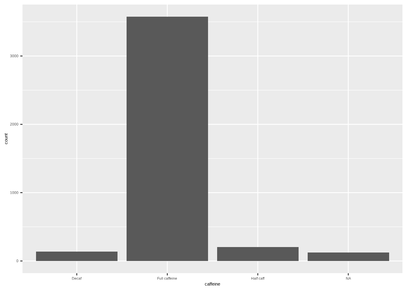
6.1.2 Relative frequency bar plot
Template (proportion):
# after_stat(prop) computes proportions within the layer
ggplot(DATA, aes(x = VAR, y = after_stat(prop), group = 1)) +
  geom_bar()
Example:
ggplot(coffee, aes(x = caffeine, y = after_stat(prop), group = 1)) +
  geom_bar()
Note
Tip: Add labels/theme as needed: labs(x = "", y = "Proportion") + theme_minimal()
6.2 Stacked bar plots
Template:
ggplot(DATA, aes(x = VAR1, fill = VAR2)) +
  geom_bar()
Example (stacked counts):
ggplot(coffee, aes(x = caffeine, fill = taste)) +
  geom_bar()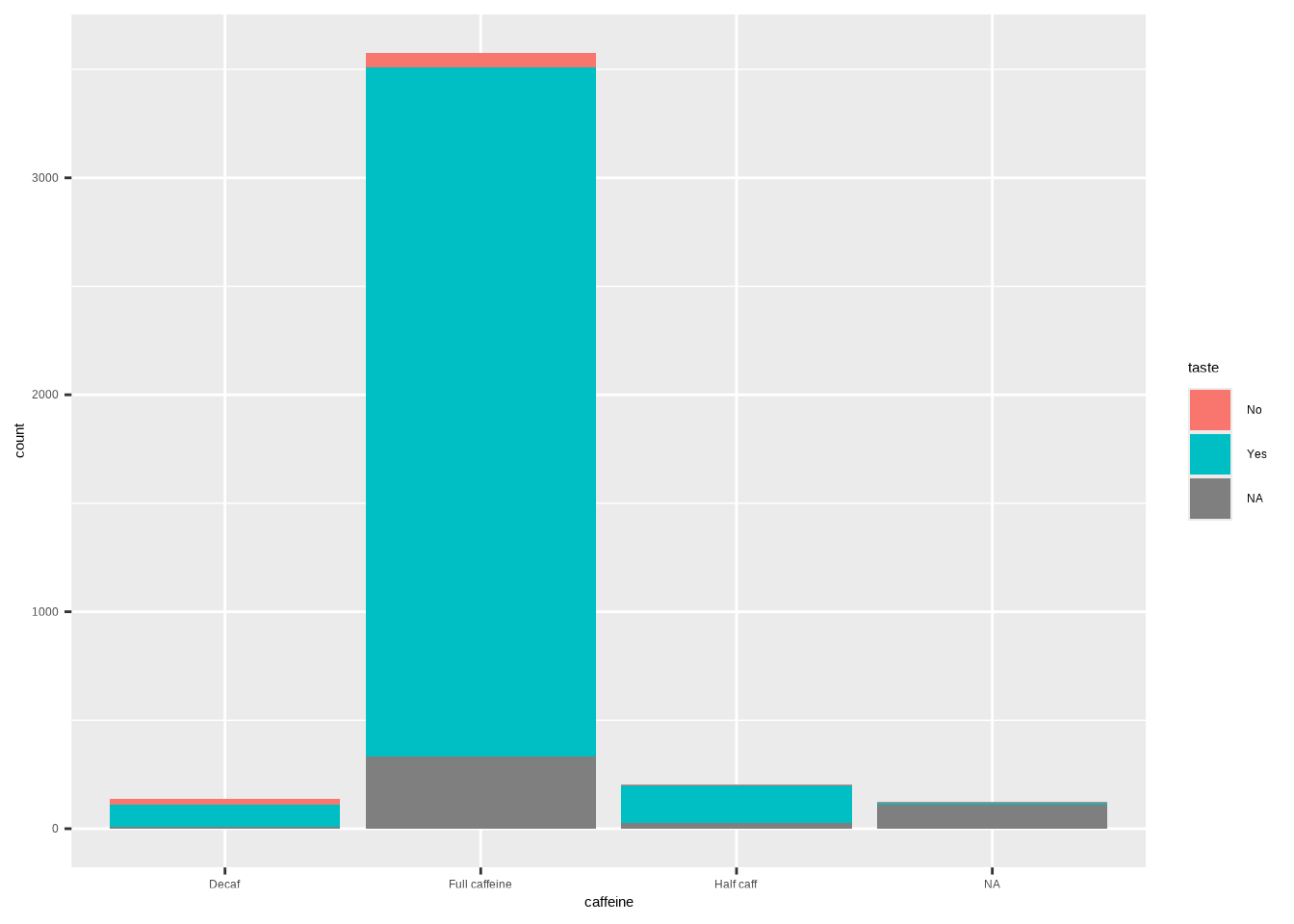
Example (horizontal):
ggplot(coffee, aes(y = caffeine, fill = taste)) +
  geom_bar()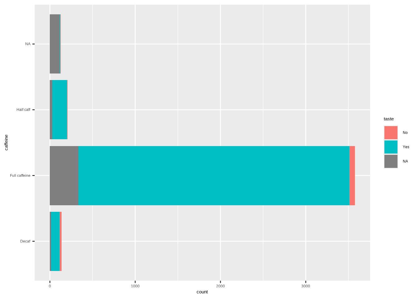
Template (stacked proportions):
ggplot(DATA, aes(x = VAR1, fill = VAR2)) +
  geom_bar(position = "fill") +
  labs(y = "Proportion")
6.3 Dodged Bar Plot
Template:
ggplot(DATA, aes(x = VAR1, fill = VAR2)) +
  geom_bar(position=position_dodge())
Example (dodged counts):
ggplot(coffee, aes(x = caffeine, fill = taste)) +
geom_bar(position = position_dodge())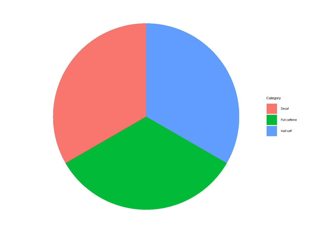
Example (horizontal):
ggplot(coffee, aes(y = caffeine, fill = taste)) +
geom_bar(position = position_dodge())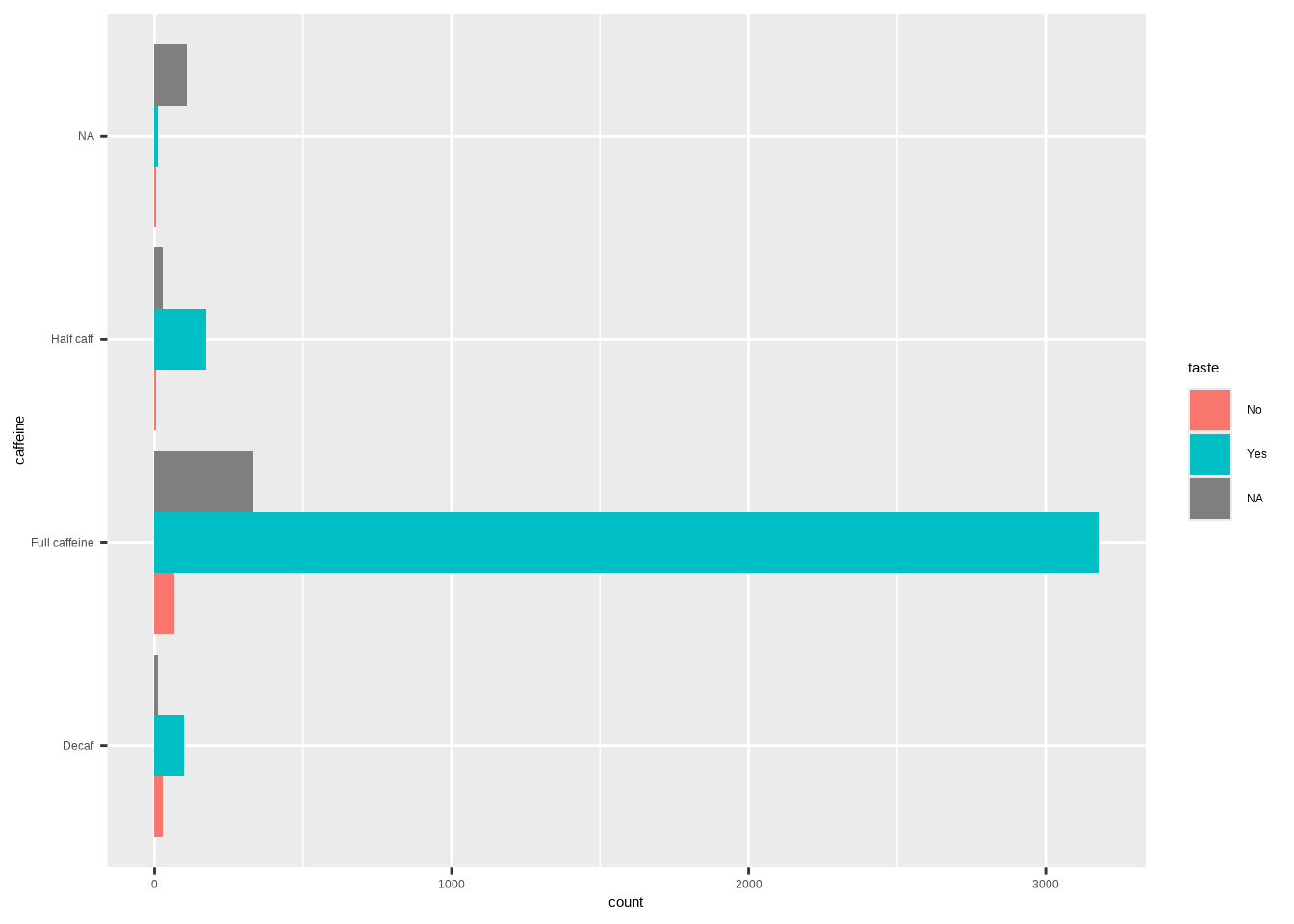
6.4 Pie charts (use sparingly)
Note: Pie charts can be harder to compare precisely than bars. If you use them, label clearly.
Template:
ggplot(DATA, aes(fill = VAR)) +
  geom_pie()
Example:
ggplot(coffee, aes(fill = caffeine)) +
  geom_pie()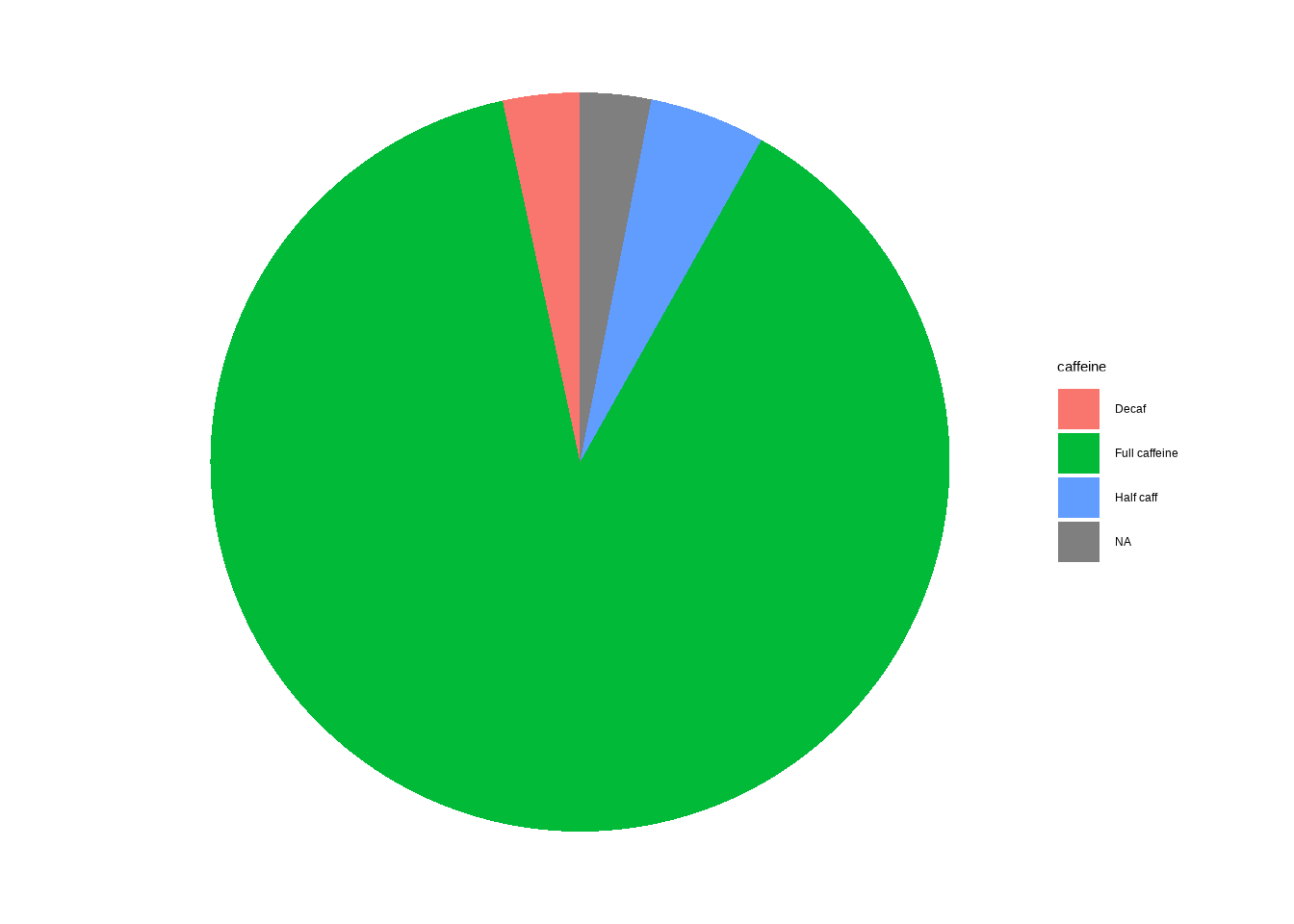
7 Appendix: minimal templates (copy‑paste)
Each template below has placeholders in ALL CAPS (e.g., DATA, VAR, VAR1, VAR2). Replace them with your own dataset name and variable names.
7.1 Frequency table
cat_stats(DATA$VAR) DATA→ the name of your dataset (e.g.,coffee).VAR→ a single categorical variable (e.g.,caffeine).
7.2 Proportions only
cat_stats(DATA$VAR, prop_only = TRUE)DATA→ the name of your dataset (e.g.,coffee).VAR→ a single categorical variable (e.g.,caffeine).
7.3 Bar Plot: Frequency
ggplot(DATA, aes(x = VAR)) +
geom_bar()DATA→ the name of your dataset (e.g.,coffee).VAR→ a single categorical variable (e.g.,caffeine).
7.4 Bar Plot: Proportion
ggplot(DATA, aes(x = VAR, y = after_stat(prop), group = 1)) +
geom_bar()DATA→ the name of your dataset (e.g.,coffee).VAR→ a single categorical variable (e.g.,caffeine).
7.5 Cross-tabulations (all)
cat_stats(DATA$VAR1, DATA$VAR2)DATA→ the name of your dataset (e.g.,coffee).VAR1→ a single categorical variable (e.g.,caffeine).VAR2→ a single categorical variable (e.g.,taste).
7.6 Cross-tabulations (proportions)
cat_stats(DATA$VAR1, DATA$VAR2, prop = "table")
cat_stats(DATA$VAR1, DATA$VAR2, prop = "row")
cat_stats(DATA$VAR1, DATA$VAR2, prop = "col")DATA→ the name of your dataset (e.g.,coffee).VAR1→ a single categorical variable (e.g.,caffeine).VAR2→ a single categorical variable (e.g.,taste).
7.7 Stacked Bar (counts)
ggplot(DATA, aes(x = VAR1, fill = VAR2)) + geom_bar()DATA→ the name of your dataset (e.g.,coffee).VAR1→ a single categorical variable (e.g.,caffeine).VAR2→ a single categorical variable (e.g.,taste).
7.8 Stacked Bar (proportions)
ggplot(DATA, aes(x = VAR1, fill = VAR2)) +
geom_bar(position = "fill") + labs(y = "Proportion")DATA→ the name of your dataset (e.g.,coffee).VAR1→ a single categorical variable (e.g.,caffeine).VAR2→ a single categorical variable (e.g.,taste).
7.9 Dodeged Bar Plot
ggplot(DATA, aes(x = VAR1, fill = VAR2)) +
geom_bar(position=position_dodge())DATA→ the name of your dataset (e.g.,coffee).VAR1→ a single categorical variable (e.g.,caffeine).VAR2→ a single categorical variable (e.g.,taste).
7.10 Pie Chart
ggplot(DATA, aes(fill = VAR)) +
geom_pie()DATA→ the name of your dataset (e.g.,coffee).VAR→ a single categorical variable (e.g.,caffeine).