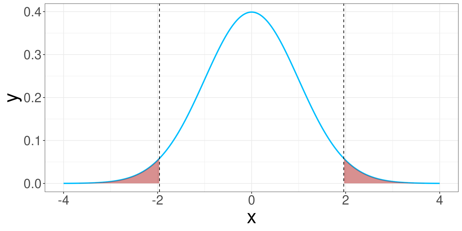
Statistical Inference

R Packages

• Tidyverse
• rcistats
• broom

Data & Motivation

• Data & Motivation

• Statistical Inference

• Hypothesis Testing

• Decision Making

• Confidence Intervals

• Regression Coefficient Inference

• Linear Regression Inference in R

• Logistic Regression Inference in R

Palmer Penguins Data

Variables of Interest

• fliper_len: Flipper Length
• body_mass: Body mass in grams

Artwork by @allison_horst

Heart Disease Data

Variables of Interest

• trestbps: Resting Blood Pressure
• disease: Indicating if they have heart disease

No Association

An Association

Association?

Association?

Association?

Statistical Inference

• Data & Motivation

• Statistical Inference

• Hypothesis Testing

• Decision Making

• Confidence Intervals

• Regression Coefficient Inference

• Linear Regression Inference in R

• Logistic Regression Inference in R

What is Statistical Inference?

• Drawing conclusions about a population based on a sample
• Population = entire group
• Sample = subset

Two Main Types of Inference

1. Estimation
2. Hypothesis Testing

We’ll be focusing on two fundamental techniques in inference. First, estimating population values (like the mean), and second, testing claims about the population.

Estimation

• Point Estimate: Single best guess (e.g., \(\hat \beta_1\))
• Interval Estimate: Range of values likely to contain the true value

Point estimates are easy but not very informative. Intervals give us a sense of uncertainty, which is critical in inference.

Key Concepts and Tools

To conduct a hypothesis test, we need to know the following:

• Sampling Distribution
• Central Limit Theorem
• Standard Error

These three concepts are foundational. Understanding them helps us assess how reliable our estimates are.

Hypothesis Testing

• Data & Motivation

• Statistical Inference

• Hypothesis Testing

• Decision Making

• Confidence Intervals

• Regression Coefficient Inference

• Linear Regression Inference in R

• Logistic Regression Inference in R

Hypothesis Tests

Hypothesis tests are used to test whether claims are valid or not. This is conducted by collecting data, setting the Null and Alternative Hypothesis.

Null Hypothesis \(H_0\)

The null hypothesis is the claim that is initially believed to be true. For the most part, it is always equal to the hypothesized value.

Alternative Hypothesis \(H_1\)

The alternative hypothesis contradicts the null hypothesis.

Example of Null and Alternative Hypothesis

We want to see if \(\beta\) is different from \(\beta^*\)

Null Hypothesis	Alternative Hypothesis
\(H_0: \beta=\beta^*\)	\(H_1: \beta\ne\beta^*\)
\(H_0: \beta\le\beta^*\)	\(H_1: \beta>\beta^*\)
\(H_0: \beta\ge\beta^*\)	\(H_1: \beta<\beta^*\)

One-Side vs Two-Side Hypothesis Tests

Notice how there are 3 types of null and alternative hypothesis, The first type of hypothesis (\(H_1:\beta\ne\beta^*\)) is considered a 2-sided hypothesis because the rejection region is located in 2 regions. The remaining two hypotheses are considered 1-sided because the rejection region is located on one side of the distribution.

Null Hypothesis	Alternative Hypothesis	Side
\(H_0: \beta=\beta^*\)	\(H_1: \beta\ne\beta^*\)	2-Sided
\(H_0: \beta\le\beta^*\)	\(H_1: \beta>\beta^*\)	1-Sided
\(H_0: \beta\ge\beta^*\)	\(H_1: \beta<\beta^*\)	1-Sided

Hypothesis Testing Steps

1. State \(H_0\) and \(H_1\)
2. Choose \(\alpha\)
3. Compute confidence interval/p-value
4. Make a decision

Walk through the steps slowly with an example in mind. Emphasize that \(\alpha\) is a threshold, not the actual probability of error.

Rejection Region

• The rejection region is the set of all test statistic values that lead to rejecting \(H_0\).

• It’s defined by a significance level (\(\alpha\)) — the probability of rejecting \(H_0\), when it’s actually true.

Rejection Region

alpha <- 0.05

# Critical values for two-tailed test
z_critical <- qnorm(1 - alpha / 2)

# Create data for the normal curve
x <- seq(-4, 4, length = 1000)
y <- dnorm(x)

df <- data.frame(x = x, y = y)

ggplot(df, aes(x = x, y = y)) +
  geom_line(color = "deepskyblue", linewidth = 1) +
  geom_area(data = subset(df, x <= -z_critical), aes(y = y), fill = "firebrick", alpha = 0.5) +
  geom_area(data = subset(df, x >= z_critical), aes(y = y), fill = "firebrick", alpha = 0.5) +
  geom_vline(xintercept = c(-z_critical, z_critical), linetype = "dashed", color = "black") 

Decision Making

• Data & Motivation

• Statistical Inference

• Hypothesis Testing

• Decision Making

• Confidence Intervals

• Regression Coefficient Inference

• Linear Regression Inference in R

• Logistic Regression Inference in R

Decision Making

Hypothesis Testing will force you to make a decision: Reject \(H_0\) OR Fail to Reject \(H_0\)

Reject \(H_0\): The effect seen is not due to random chance, there is a process contributing to the effect.

Fail to Reject \(H_0\): The effect seen is due to random chance. Random sampling is the reason why an effect is displayed, not an underlying process.

Decision Making: P-Value

The p-value approach is one of the most common methods to report significant results. It is easier to interpret the p-value because it provides the probability of observing our test statistics, or something more extreme, given that the null hypothesis is true.

If \(p < \alpha\), then you reject \(H_0\); otherwise, you will fail to reject \(H_0\).

Significance Level \(\alpha\)

The significance level \(\alpha\) is the probability you will reject the null hypothesis given that it was true.

In other words, \(\alpha\) is the error rate that a researcher controls.

Typically, we want this error rate to be small (\(\alpha = 0.05\)).

Confidence Intervals

• Data & Motivation

• Statistical Inference

• Hypothesis Testing

• Decision Making

• Confidence Intervals

• Regression Coefficient Inference

• Linear Regression Inference in R

• Logistic Regression Inference in R

Confidence Intervals

• A confidence interval gives a range of plausible values for a population parameter.
• It reflects uncertainty in point estimates from sample data.

Interpretation

“We are 95% confident that the true mean lies between A and B.”

• This does not mean there’s a 95% chance the mean is in that interval.
• It means: if we repeated the sampling process many times, 95% of the intervals would contain the true value.

This is one of the most common misconceptions. Clarify that the confidence is in the method, not any one interval.

Factors Affecting CI Width

• Sample size (\(n\)): larger \(n\) → narrower CI
  
• Standard deviation (\(s\) or \(\sigma\)): more variability → wider CI
  
• Confidence level: higher confidence → wider CI

Use this to summarize what controls how “precise” our confidence interval is. Give examples of each.

Decision Making: Confidence Interval Approach

The confidence interval approach can evaluate a hypothesis test where the alternative hypothesis is \(\beta\ne\beta^*\). The confidence interval approach will result in a lower and upper bound denoted as: \((LB, UB)\).

If \(\beta^*\) is in \((LB, UB)\), then you fail to reject \(H_0\). If \(\beta^*\) is not in \((LB,UB)\), then you reject \(H_0\).

Regression Coefficient Inference

• Data & Motivation

• Statistical Inference

• Hypothesis Testing

• Decision Making

• Confidence Intervals

• Regression Coefficient Inference

• Linear Regression Inference in R

• Logistic Regression Inference in R

Testing Association

\[ Y = \beta_0 + \beta_1 X \]

In an equation, the coefficient multiplied (\(\beta_1\)) to the variable \(X\) determines if there is an association between \(X\) and \(Y\).

Coefficient Inference

No Association

\[ \beta_1 = 0 \]

Association

\[ \beta_1 \ne 0 \]

Hypothesis Test

Null Hypothesis

\[ H_0:\ \beta_1 = 0 \]

Alternative Hypothesis

\[ H_1:\ \beta_1 \ne 0 \]

Testing Association

\[ Y = \beta_0 + \beta_1 X_1 + \beta_2 X_2 + \beta_3 X_3 \]

In an equation, the coefficient multiplied (\(\beta_2\)) to the variable \(X_2\) determines if there is an association between \(X_2\) and \(Y\).

Hypothesis Test

Null Hypothesis

\[ H_0:\ \beta_2 = 0 \]

Alternative Hypothesis

\[ H_1:\ \beta_2 \ne 0 \]

Linear Regression Inference in R

• Data & Motivation

• Statistical Inference

• Hypothesis Testing

• Decision Making

• Confidence Intervals

• Regression Coefficient Inference

• Linear Regression Inference in R

• Logistic Regression Inference in R

Conducting HT of \(\beta_j\)

XLM <- lm(Y ~ X, data = DATA)
tidy(XLM)

• XLM: Object where the model is stored
• Y: Name of the outcome variable in DATA
• X: Name of the Predictor Variable(s) in DATA
• DATA: Name of the data set

Example

Is there a significant relationship between penguin body mass (outcome; body_mass) and flipper length (predictor; flipper_len)? Use the penguins data set to determine a significant association.

Example

m1 <- lm(body_mass ~ flipper_len, 
         penguins)
tidy(m1)

#> # A tibble: 2 × 5
#>   term        estimate std.error statistic   p.value
#>   <chr>          <dbl>     <dbl>     <dbl>     <dbl>
#> 1 (Intercept)  -5781.     306.       -18.9 5.59e- 55
#> 2 flipper_len     49.7      1.52      32.7 4.37e-107

95% Confidence Interval

tidy(XLM, 
     conf.int = TRUE)

• XLM: Object where the model is stored

X% Confidence Interval

tidy(XLM, 
     conf.int = TRUE, 
     conf.level = X)

• XLM: Object where the model is stored
• X: A number between 0 and 1 to specify confidence level

Example

tidy(m1, 
     conf.int = TRUE, 
     conf.level = 0.9)

#> # A tibble: 2 × 7
#>   term        estimate std.error statistic   p.value conf.low conf.high
#>   <chr>          <dbl>     <dbl>     <dbl>     <dbl>    <dbl>     <dbl>
#> 1 (Intercept)  -5781.     306.       -18.9 5.59e- 55  -6285.    -5276. 
#> 2 flipper_len     49.7      1.52      32.7 4.37e-107     47.2      52.2

Logistic Regression Inference in R

• Data & Motivation

• Statistical Inference

• Hypothesis Testing

• Decision Making

• Confidence Intervals

• Regression Coefficient Inference

• Linear Regression Inference in R

• Logistic Regression Inference in R

Conducting HT of \(\beta_j\)

XLM <- glm(Y ~ X, 
           data = DATA, 
           family = binomial())
tidy(XLM)

• XLM: Object where the model is stored
• Y: Name of the outcome variable in DATA
• X: Name of the Predictor Variable(s) in DATA
• DATA: Name of the data set

Example

Is there a significant association between heart disease (outcome; disease) and resting blood pressure (predictor; trestbps). Use the heart_disease data set to determine a significant association.

Example

m1 <- glm(disease ~ trestbps, 
          data = heart_disease, 
          family = binomial())
tidy(m1)

#> # A tibble: 2 × 5
#>   term        estimate std.error statistic p.value
#>   <chr>          <dbl>     <dbl>     <dbl>   <dbl>
#> 1 (Intercept)  -2.49     0.905       -2.76 0.00586
#> 2 trestbps      0.0177   0.00681      2.61 0.00914

Confidence Interval

tidy(XLM, 
     conf.int = TRUE, 
     conf.level = LEVEL)

• XLM: Object where the model is stored
• LEVEL: A number between 0 and 1 to specify confidence level
• defaults to 0.95

EX: 95% Confidence Interval

tidy(m1, 
     conf.int = TRUE)

#> # A tibble: 2 × 7
#>   term        estimate std.error statistic p.value conf.low conf.high
#>   <chr>          <dbl>     <dbl>     <dbl>   <dbl>    <dbl>     <dbl>
#> 1 (Intercept)  -2.49     0.905       -2.76 0.00586 -4.31      -0.747 
#> 2 trestbps      0.0177   0.00681      2.61 0.00914  0.00461    0.0314

Odds Ratio & Confidence Intervat

tidy(XLM, 
     exponentiate = TRUE, 
     conf.int = TRUE)

• XLM: Object where the model is stored

Example

tidy(m1, 
     exponentiate = TRUE, 
     conf.int = TRUE)

#> # A tibble: 2 × 7
#>   term        estimate std.error statistic p.value conf.low conf.high
#>   <chr>          <dbl>     <dbl>     <dbl>   <dbl>    <dbl>     <dbl>
#> 1 (Intercept)   0.0826   0.905       -2.76 0.00586   0.0135     0.474
#> 2 trestbps      1.02     0.00681      2.61 0.00914   1.00       1.03